New website details

Please visit at my new home...

http://www.aptc.co.za

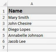
Customising shapes

This post was inspired by my child's project last week.  She was listing some interesting facts about her topic - easy enough - but she wanted them to be typed into "cacao pod" shapes.  Obviously.

Now, you are probably quite comfortable with creating basic shapes in MS Office applications but did you know you can now customise those shapes to suit your exact shape requirements?

• First, you need to insert a basic shape that is reasonably similar to the ultimate shape you would like to create.
• Next, right click over the shape and choose Edit Points.
• The shape will now be highlighted in red with black markers to indicate where the points are.
• Place your mouse pointer over an edit point marker and click and drag to amend the original shape.
• Once you are satisfied with the new shape, click anywhere else to deselect the shape.

That's it - facts typed into cacao bean pod shapes ready to stick onto a cacao tree project.

As always, please share if you think someone else may find this useful and let me know if there are any other tips, tricks or tutorials you'd like to see featured on this blog.

Where is the bottom border?

Working with tables in MS Word can make many of your documents much easier to manage.  However there are occasions when even the simple-to-use tables can be frustrating. One frequent frustration that many people face is:

"Why has the border not printed at the bottom of my table"

Well, that's because borders only appear at the end of a row (and I'm going with the assumption that borders have been switched on) 

So, if a row contains a reasonable amount of information, there may come a time when it can't physically fit all that info onto the space available at the bottom of the page, and just like any other text, as soon as MS Word runs out of space it adds a new page.    As you have not inserted a new row, MS Word will NOT draw a border to indicate the end of the row, because, well.... it hasn't reached the end of the row.

Of course this is all well and good, but it just doesn't look very nice, does it?

Instead of trying to manually shift your information around - or the even more common sin of reducing font size to force the information to fit - you can simply instruct MS Word to not allow the row to split between pages.

Position cursor in the row that you want to stop breaking over two pages

• Select the Layout tab in the Table Tools ribbon

• Click the Properties button 

• Click on the Row tab and deselect the option Allow row to break across pages

• Click OK

That's it.  Neat and tidy without too much effort from you - especially not mismatched font sizes trying to force.

Hope this was helpful. As always...share if you think someone else might find this beneficial, or leave a comment if there is anything else you'd like to see featured here.

Using Indents in MS Word

Indents are something which seem to leave many people baffled, and yet if you get to know how to handle them, you'll be surprised how easy and useful they are.  If you've ever found your self tabbing or pressing the space bar numerous times to shift your text over then this is post for you.

Typically your text is typed within the boundaries of the margins, however margins are set for the entire document and you may want to adjust the margins for only a small section of your document.  In this case you can make use of Indents.

Indents are used to align blocks of text by creating left and right boundaries for selected paragraphs without having to change margins for the whole document.  There are four indent markers positioned at the edges of the horizontal ruler as depicted below:

Moving the First Line Indent moves the text on the first line of the paragraph in line with the indent, but the remaining lines of the paragraph adhere to the margin settings.

Moving the Hanging Indent moves the text on everything except the first line of the paragraph.

Moving the Left Indent moves all the text within the paragraph to the match the indent settings.

Remember that each line within a document can have its own indent settings, so to ensure that your indent changes take effect to the required areas, make sure you have selected each line that requires the indent changed.

Don't be afraid to play around with the indents to see the changes they can make - save regularly when you're happy with a change, and press Undo when you're not :) and of course -please share this if you think it could be of value to someone else

How to add a password to an Excel file

You may want to add a password to a file if you are storing sensitive data on a USB drive, emailing it to others, or you just want to add an extra layer of security to a file on a shared network drive.

• Select Save As
• Specify the file name and location as normal.  If the file is an existing file, leave the current information in place
• Click the Tools drop down list
• Choose General Options…

• Enter the password(s) you would like to use. (You may use one or both passwords as required)

1. Password to Open – This password will be required every time the file is opened.
2. Password to Modify – This password will be requested when you open the file. Without the password you still have the option to select the Read Only button to open the file without saving privileges. 

• Click OK and reconfirm password(s).

Please don't forget the password you have allocated to the file though - here is the official Microsoft stance

"Excel lets you password protect your workbooks, and your worksheets. But, it's easy to forget or misplace your passwords. Unfortunately, if that’s happened to you, we don’t have a way to help you recover a lost password.
Excel doesn't store passwords where you or Microsoft can look them up. That's also true for the other Office programs that let you protect files. That's why it's always a good idea to store your passwords someplace safe.
Some third-party companies offer programs for unlocking files. For legal reasons, we can't recommend those programs. You can try them, but at your own risk."

http://office.microsoft.com/en-001/excel-help/recover-a-password-to-open-a-workbook-or-worksheet-HA102809703.aspx

Getting VLOOKUP to return multiple values

This post is for the somewhat more advanced Excel user.

You may already be familiar with the VLOOKUP function, what you may not know is that you can get a single VLOOKUP formula to return multiple values by using an array.

1. Select each cell that you want to contain a result from the VLOOKUP.  In the screenshot below, the cells I4:K4 were selected
2. Switch to the Formulas tab, select Lookup&Reference, VLOOKUP
3. Specify the Lookup_value and Table_array as normal
4. Enter a column number for each column that you want data returned from.  Separate the column numbers by commas and enclose it all in braces / curly brackets {  }.  The column numbers can be specified in any order.  In the example below, data will be returned from columns {5,6,3}
5. Specify your Range_lookup requirements
6. Press CTRL, SHIFT, ENTER

Hope this is a time saver for you!  Please share if you think anyone might find this useful too.

Restrict values using Data Validation lists

Using the Data Validation feature in Excel you are able to restrict entry to a predefined list of values.  

In many cases spreadsheets are completed by more than one user which often results in different styles of inputting data.  By having a drop down list to select from ensures consistency which not only makes for a neater appearance, but also significantly improves the ease of use of tools such as Pivot Tables and Filters.

• Somewhere in your spreadsheet, type out the list of values that you would like to use as the source for your drop down list 
• Select the cells to which you would like to add Data Validation drop down list
• On the Data tab, select Data Validation. (A drop-down menu will appear.)
• Select Data Validation.
• Select List from the Allow drop down.
• In the Source field, select the range of cells that will act as the source data for the drop down list

• Click OK and begin using the drop down list to aid data entry

Happy spread-sheeting! Please share if you found this useful.

Easy way to wrap text in MS Excel

When you want to split your heading over more than one line but within the same cell, you may be familiar with the Wrap Text button on the ribbon.  However there is a quicker method that can be implemented as you are typing: ALT Enter.

Using the example below, type Stock then press ALT ENTER to move your cursor into the next line, then type MVMT and press ALT ENTER to move down again and then type Boxes.  Press ENTER when you are done.

You can even edit a cell afterwards to add a line break if necessary, you'd just have to press ALT ENTER at the appropriate spot in the formula bar (or in the cell itself if you're in edit mode).

Please share this using one of the buttons below if you think others will find this useful, or leave me a comment if there is something else you'd like to learn about.

Non breaking spaces in MS Word

Perhaps you've heard of non breaking spaces, perhaps not, but you certainly should know how to use them.

On occasion you may want to override the way MS Word wraps text at the end of a line.  For example, you may want a person's name and surname to always appear on the same line or perhaps the date and year are separating and you'd prefer they didn't.

Looking at this example the name (which I've highlighted to make it easier to spot) has wrapped onto two lines.

In order to force MS Word to keep the name and surname together, I've replaced a normal space between the name and surname with a non breaking space.  Easily done.  Simple replace the existing space with CTRL SHIFT SPACEBAR

Whilst this is not something you're likely to use on a very frequent basis, it's a great little trick to know.

Formula Auditing in Excel

When you're viewing a formula, you would typically read the formula bar to determine which cells the formula uses, and this is where the distinct blue arrows of Formula Auditing make your life a lot easier.  

First, select a cell that contains a formula, then switch to the Formulas tab on the ribbon.   In the Formula Auditing group, click the Trace Precedents button.

Trace Precedents will send a blue arrow to all of the cells which are used in the creation of the formula that is currently selected.

If the cell that is selected does not contain a formula the Trace Precedents error alert will appear.

If you'd like to find out if a cell is required elsewhere on the spreadsheet, click the Trace Dependents button.  If the cell is used by any other calculation, a blue arrow will direct you to that value.

At any stage you can use the Remove Arrows button to clear the arrows on your screen.

This really is any easy way to figure out how your spreadsheets are inter linked, I certainly use it often when faced with assisting someone else with their Excel files - it helps me get to grips with their spreadsheets in half the time.

Using Quick Calculations

The status bar appears at the bottom of the Excel window and you are most likely familiar with finding settings like your zoom control here.  Naturally, there is far more use to the status bar than just zooming, and one of those things is activating the quick calculations.

These quick calculations are useful when you want to spot check values but don't necessarily need the resulting value to be placed as an independent value on the spreadsheet.

Right click onto the status bar.  This will display all the content that you could have displayed if you wish.  There is a section that is specifically for the quick calculations - typically Sum is already selected.  You may select any calculation types you like.

When you next select a range of cells containing values, the status bar will display the quick calculations that you have requested.

Calculating a loan repayment with the PMT function

Here's an Excel function we could all make use of.  Calculating the repayment on a loan.

In order for this calculation to work, you require 3 items:  the amount being borrowed; the interest rate that will be charged; and the term over which the loan will be re-payed.

First layout your spreadsheet with the required information, and click into the cell that you would like the answer (i.e. the monthly installment) to appear.  Now switch to the Formulas tab on the ribbon, and from the Financial list scroll down to find the PMT calculation.

The Function Arguments window will appear with 3 required fields (for the information that you have ready) and 2 further optional fields that I'll explain a little further down.  A clue to indicate which fields are required vs which are optional, is that the required fields have a bold title.

Place your cursor into the first required field, Rate, and click once on the cell that contains your interest rate value.  Typically the interest rate that you are quoted is the APR (Annual Percentage Rate) and as such the amount is what you will be charged per year.  Because we are attempting to calculate the monthly installment, we need to give Excel the monthly interest rate.  You are able to do so by dividing this APR value by 12.

Now place your cursor into the second required field, Nper.  This field represents the total number of installments you will be paying.  So if your loan is taken out over a 10 year period, you won't be making 10 payments in total, but rather 10 years of 12 months each, so a total of 120 payments.   Click once onto the cell that contains your term value, and then type *12

The final required field is PV.  This part of the calculation is where you indicate the PresentValue i.e. the loan amount that needs to be re-payed.  Ensure that your cursor is in the PV field, type a minus sign and then click once onto the cell on your spreadsheet that contains the loan amount.  Typing a minus sign is not required, but it's a clever way to ensure that the calculated monthly repayment does not appear as a negative value.
At this point you can click OK to see installment that will be required for this loan.  Please remember that many loan companies will have their own additional costs that will mean this will not be an exact amount but it will at least give you a good idea of what to expect.

There are however, two additional fields are not required in order for the calculation to work correctly, but they can have an impact on the answer.

The first of these fields is FV.  This is the FutureValue - the amount that the loan needs to reach by the end of the loan period.  This would typically be zero - you want to pay the loan off in full over the course of the loan period and if you leave this field blank, Excel will assume you wish to pay off the entire loan.  Of course this isn't always the case, and sometimes your loan may allow for what is known as a balloon payment / residual payment.  If you have such a balloon payment, you still enter the full loan amount into the PV field, and the balloon amount into the FV field.

The second optional field is Type.  This is used to indicate when payment is required - if you are required to pay at the end or beginning of the period.  Simply put, is your payment due at the end of the month or beginning.  If you leave this field blank, it is assumed you pay at the end of the month.  You can enter a 1 to indicate payment is due at the beginning of the period, whilst a 0 indicates payment at the end of the period.

I'm wondering if this post was heavy reading for you?  Would you prefer to have seen this tutorial as a 2 or 3 minute video clip?  Let me know you're thoughts

Using the Text to Columns wizard

To separate the data of one Excel cell into separate columns, you can use the 'Convert Text to Columns Wizard'. 

Using this example, I'll show you how to separate a list of full names into last and first names.

First, select all the data you want to separate, then on the Data tab of the ribbon, click Text to Columns

A wizard window will appear with some prompts that will guide you through this process.  The first of which is deciding if your data is Delimited or Fixed width.  Basically, Excel needs to know where the data should be split... should it chop the data after a fixed number of characters (Fixed width) or when it finds a specific character (Delimited).  In the case of names and surnames, you cannot predict how long a name will be, and therefore it makes sense to use Delimited.  

Click Next

Now you get to indicate what the delimiter is.  Check boxes have been created for the most common characters that act as delimiters.  In this example a space separates the name from the surname and has been checked as such.  If necessary, you can click the Other option and type in the delimiter.  

This screenshot shows an example of needing to use a colon (:) as the delimiter.

As soon as the delimiter is specified, you can see a preview of your data below. Click Next and then click Finish to see your newly separated data.

Another example is of data the suits a Fixed width delimiter.  This should only be used when you are certain of the number or characters you'd like between each section of data.

Once again, select all your data first, then on the Data tab of the ribbon click Text to Columns.  Choose Fixed width as your delimiter and click Next

You now create"break lines" which show where the data is to be separated by following the instructions at the top of the window.  Once you've indicated all the break lines click Next.

In the case of this example, I've separated the actual digits of the serial number away from the text "S/N" and actually I don't want the "S/N" heading anyway, so this step gives you the option to dump any columns of data you don't require.  Click the column that you don't want to keep (it'll be selected very clearly in black) and then click the option at the top of the window "Do not import column (skip)"

Click Finish to see your data.

That's it.  Quite an easy process once you get the hang of it.  Now you'll never need to manually edit those spreadsheets when next faced with a scenario like this.

Have a great week!

Paste data using the Transpose feature in MS Excel

I don't know about you, but I often lay out data on a spreadsheet and then change my mind about the orientation of it.  Thankfully there is a quick and easy way to get MS Excel data to swap places - basically putting all your row data into columns and your column data into the rows.

This is what your data may look like to begin with.

Highlight all the information and Copy.  You'll see the ubiquitous "sparkling lines" appear around the data to confirm you've copied successfully.  Now place your cursor into any other empty cell and choose Paste. I do this by right clicking over the cell, but you can also click the Paste button on the Home tab of the ribbon.

From the Paste Options list, select the Transpose icon.  That's it!  Your data will now appear transposed perfectly.

A quick note...you can't use the CTRL V shortcut key to paste as this will not show you the Paste Options buttons nor can you cut the original data and perform a Paste Transpose.

More Excel tips and tricks coming your way soon.  Let me know if there is anything in particular you're hoping to see.

My favourite ways to select text in MS Word

There are so many ways to select text, and we all have our favourites.... these are mine.

• a single word - double click over the word.
• an entire sentence  - Hold CTRL and click once anywhere on the sentence.
• the entire document - Press CTRL A
• a paragraph - triple click anywhere within the paragraph
• Irregular area - click once at the beginning of the area, hold your SHIFT key and then click at the end of the area to be selected

It's been a very MS Word focused set of tips over the last few weeks.  I hope you've found them useful, please share if you have.  I'll be working on some Excel tips next.

How to hide page numbering on the first page of a MS Word document

You may not want to have page numbers appear on the first page of your document, particularly if it is a cover or summary page.

Click on the Insert tab of the ribbon, and choose Page Number - my preference is to then select Bottom of Page, but you may place the page number as you prefer - next, scroll through the list and select the style of page number you would like to use.

Once you have made your selection, you will enter "Header & Footer mode".   You will notice a few things:

- Your document text will appear greyed out
- Your cursor will appear in a demarcated area with a grey tag on the left titled Footer
- There will be an additional ribbon tab (highlighted in green) and titled Header & Footer Tools

On the Header & Footer Tools Design ribbon tab, click the check box for Different First Page.

The footer area at the bottom of the first page will now be titled First Page Footer and the page number will automatically be removed.

At this point you could add a different piece of text to appear as the first page footer, alternately live it blank. Once you have completed customisation of the footer space, you should exit and return to working in the document as normal by either clicking the Close Header and Footer button on the Design tab, or even quicker, double click anywhere on the document outside the demarcated footer area.

Do you have any other Header & Footer related questions?  Let me know by adding a comment and I'll create a post especially for you.

Forward multiple emails to single recipient

Sometimes you need to forward many emails to another person.   Mostly people tend to do this one by one, which can be time consuming for the sender, and possibly annoying for the recipient who is suddenly faced with an ever increasing number of unread messages in their mailbox (and that's not even considering the delights of extra beeps on the mobile phone)  Fortunately there is a better way!

Open Outlook.  Select the first message you would like to forward.  Hold the CTRL key and select each subsequent message you would like to forward.

On the Home tab, click the Forward button.

A new email message window will appear, and each of the selected email messages are added to it as attachments.    You can now continue to address and send your email as normal.

Problem solved.  One physical email forwarded, and it contains all the other related items attached within it.

Useful? Anything else you'd like to learn about?  Let me know, or share this by using the links below.

Adding captions in MS Word

If you are writing a long MS Word document containing a lot of images, tables or other graphical items, it is preferable, and sometimes required, to add captions to those items in order to be able to easily reference them by their number in the text as well as generate a Table of Figures.

To add a caption, select the item to be captioned in your document and click the References tab.  In the Captions section, click Insert Caption.  (You could also right click over the item and choose Insert Caption from the menu.)

The Caption dialog box will appear with selections to make for the captioning style you would like to use.

The first field in the dialog box (titled Caption:) displays what the caption would look like if you inserted it at this point.  Beneath this are the options you may choose from.  The Label you want should ideally denote the type of item you are captioning.  For example, if you have inserted a Table, then choose the Table label.  Once you have decided on the label you would like to use, then decided on where the caption should appear in relation to the item (Above selected item or Below selected item). 

By default, captions will be numbered sequentially, if you prefer another style, click the Numbering... button to make your selection.  To change the numbering on the caption, click Numbering and make your selection from the formats available, then click OK

Remember to check the caption preview (which appears as the first field in the Caption dialog box) and once you are satisfied with your selections, click OK to insert. 

Happy captioning!

Creating Random text in MS Word

Have you ever found yourself wanting to test a new format or design in a MS Word document but feel too nervous to use your real files "just in case".

I frequently need to test things out, but don't want the hassle of typing out a few paragraphs of text, of course I could search online for something to copy...but then I just end up getting distracted.

Fortunately, somebody who works at Microsoft has clearly had this problem too, and has given us an amazingly simple solution.  Type

=Rand()

into your MS Word document and you'll instantly get about half a page of text ready for you to use!

Now you have no more excuses to practice all the tips & tricks I'll be providing!  Go on... spread the word by clicking one (or all) of the sharing buttons below.

Removing all hyperlinks in a Word document

Nowadays we get so much information from other sources, but when we paste that data into Word documents, it often pastes with the hyperlink included.  You know... all blue and clickable as displayed in the picture below.

You probably know how to remove the hyperlinks by right clicking over them, but that can become tedious when you have quite a few spread throughout a long document.

An easy way to remove all hyperlinks is to press “Ctrl+A” which will select everything in the entire document, then press "Ctrl+Shift+F9"

This will remove all of the hyperlinks whilst still keep the original format of the text.

Let me know if there are any other topics you'd like to see featured in this Tips and Tricks blog and feel free to share this with others you think may find it useful.

Using Sparklines

A sparkline is a very small line or bar chart, but, unlike typical charts which are designed to show as much information as possible and are separate to the data (in some cases even on a different sheet) sparklines fit into a single cell allowing them to appear immediately alongside the data for greater impact.

• Click on the Insert tab on the ribbon and choose one of the sparkline styles.
• Highlight the cells containing the data for the sparkline and specify where you would like sparkline to appear.
• Click OK

Once the sparkline is in place, you will have an additional tab on the ribbon called Sparkline Tools, with all the formatting options available.

Are there any other Excel tips and tricks that you'd like to see next?  Let me know by leaving a comment and don't forget to share this post with others by using the buttons below.

How to add public holidays to your Outlook calendar

Many of us use the Outlook calendar to keep track of meetings and events, as well as birthdays and anniversaries of family and friends.  Rather less known is that you are able to add public holidays into your calendar in a few quick clicks.

Click the File tab and then choose Options from the menu list.

On the Outlook Options dialog box, click Calendar in the menu list on the left.  In the Calendar options section, click Add Holidays.

The Add Holidays to Calendar dialog box displays. Select the check boxes for the countries and/or religions whose holidays you want to add to your calendar. Click OK.

Click OK again to exit the Outlook Options window.  All the holidays for the countries and /or religions you have selected will now be entered into the calendar.

That's it.  Quick and easy.  Now go book your holiday!

Quickly reverse formatting in MS Word

I often come across people who say they "hate MS Word" as "it never does what I want".  And to be fair, their documents are misbehaving, but often this is caused by formatting errors.  And I'm not referring to using Bold or Italics in the wrong places.  MS Word has all sorts of format settings, (many of which can be a bit obscure if you don't know where or what to look for) which relate to paragraph spacing, or indents, or line breaks.

As you work on and edit a document you may be deleting text, or removing visible formats (colour, bold, italics etc.) but you may be leaving a footprint trail of non-visible formats.  Some of which will drive you insane when you can't figure out why that line of text won't move down, or why your automatic numbering won't indent.

  

To ensure that you have made a clean break from any formatting that may be present, use the Clear Formatting button on the Home tab

Do you face any challenges with your MS Word documents?  Leave a comment and let me know... you might be inspiration for the next installment of MissusMcK's tips